Showing posts with label simulation. Show all posts

Sunday, July 01, 2007

Logo 也 3D

Welcome to StarLogo TNG

前陣子 survey 描述機器動作的程式語言時,看到幾個賣像不錯的 Robot 產品,竟不約而同地,都說 Logo 語

經過一連串的 google 、到處點閱後發現:原來 Logo 早已跳出原先的認知,不再只是給小朋友玩的烏龜繪圖了!

一直以來,我對 Logo 語言並不陌生,因為手邊好些科普書都有提到,例如:

  • 電腦如何思考》p53 ,Hillis 以 Logo 為例子,說明程式語言的威力;
  • 沙地上的圖案》p136 ,〈作為藝術家的烏龜,The turtle as artist〉這節說明了 Papert 的 Logo 及其 Turtle Geometry
  • MIT 媒體實驗室》p181 ,提到了控制 LEGO 積木的 Logo 語言;
  • 遊習世紀》p101 ,提到用 Logo 控制的實體機器烏龜如何幫助小孩子學習;
  • ……

Logo 語言我原先比較有印象的,就是它的烏龜繪圖。其最早的版本是一隻地板上亂逛的同時,還會以隨身攜帶的畫筆留下足跡的實體機器龜;後來這隻機器烏龜離開了地面,爬上了螢幕,變成一隻賣弄光影的傢伙。

現在一些 Logo 版本(例如 StarLogoNetLogo 等),允許同時有成百、上千隻烏龜。這些烏龜還可以依行為不同而有不同族系(例如:有些化身成兔子,有些化身成狐狸等)。這下子可以拿 Logo 來跑有大量 agents 的模擬實驗了,這裡是一些例子

此外,最新的 Logo 方言(例如 StarLogo TNG),已經讓烏龜的生活環境,由原本 2D 的平面,躍升到 3D 立體空間了。這下子光是搞搞模擬就太遜了,乾脆拿來寫些小遊戲,豈不是更酷!

如果現在還有人覺得 Logo 是小孩子玩意,是個跟不上時代的古董。這裡建議一定要去看看 Elica ,它是 Logo 另一個方言,支援 OOP ,不但有優雅的語言內涵,且也用於精緻的 3D 繪圖

如果還覺得意猶未盡的,強烈建議去閱讀閱讀 Brian Harvey 的《Computer Science Logo Style》。這本書共有三卷,且有電子檔可供下載:

  1. Symbolic Computing
  2. Advanced Techniques
  3. Beyond Programming

Tuesday, August 29, 2006

Graph-based Modeling on Python

Agent-based modeling 的電腦實驗,最核心的架構不外乎一個大迴圈(super loop)包裹著一群規則。大迴圈每跑一輪,系統就更新一次狀態,就如同時鐘的滴答(tick)聲般。通常系統每次滴答都會收集一次統計資料。這類實驗,有許多現成的 famework 可用,如最經典的 Swarm 及其後進 Repast ,還有我模仿 Repast ,自己搞的一個 ,它們都提供了 start, pause, stop 等流程控制的介面。

模擬複雜網路,也可以套用 Agent-based modeling 架構。不過諸如網路的群聚度(clustering coefficient, C)及網路特徵的路經長度(characteristic path length, L)等統計數據計算需耗費的時間,隨著網路的規模成長很快,所以不適合運作太頻繁。但我們卻得靠這些統計數據來判斷網路是否收斂、試驗是否該終止了,想試驗各個參數排列組合時,更是雪上加霜。

透過 Intermediate File 是很直覺的解法。程式每次執行都餵入一個輸入檔來初始網路結構,並以參數決定 super loop 要跑幾次。統計數據只在程式要結束時計算,然後將網路狀態及統計數據吐給輸出檔。下次要執行,就以這個輸出檔當作新的輸入,然後一樣決定要跑幾圈,最後得到另一個輸出檔。採取接力的方式,不用每次都從頭跑,不會浪費先前程式執行的時間。

Multithread 是另一個可行作法。採用 Agent-based modeling framework 的方式,一個 thread 跑核心的規則。另一個 thread 則控制試驗的流程,讓 user 決定何時該暫停下來,計算統計數據,然後決定是否繼續執行。

Dynamic Programming Language 是這次的正解。利用動態程式語言,如 Python ,可以很方便於執行時期控制模擬試驗的程式流程。我就是採用 Python ,搭配 NetworkX 來處理 Graph ,並以 matplotlib 來繪製圖表。接下來就看看如何架設這個試驗平台:

  1. 下載 Python Enthought Edition 的 installer 。它是 Python 的加強版,除了 Python 基本工具外,還整合了許多有用的工具,例如 matplotlib
  2. 這裡下載 NetworkX 的 installer 。
  3. 依序執行這兩個 installer 。

裝好了後,就以 Emergence of a small world from local interactions: modeling acquaintance networks 裡描述的實驗來操刀,試寫第一個 Python 程式:

1
2
3
4
5
6
7
8
9
10
11
12
13
14
15
16
17
18
19
20
21
22
23
24
25
26
27
28
29
30
31
32
33
34
35
36
37
38
39
40
41
42
43
44
45
46
47
48
49
50
51
52
53
54
55
56
57
58
59
60
61
62
63
64
65
66
67
68
69
70
71
72
73
74
75
76
77
78
79
80
81
82
83
84
85
86
87
88
89
90
91
92
93
94
95
96
97
98
99
100
101
102
103
104
105
106
107
108
109
110
111
112
113
114
115
116
117
118
119
120
121
122
123
124
125
126
127
128
129
130
131
132
133
134
135
136
137
138
139
140
141
142
143
144
145
146
147
148
149
150
151
152
153
154
155
156
157
158
159
160
161
162
163
164
165
166
167
168
169
170
171
172
173
174
175
176
177
178
179
180
181
182
183
184
185
186
187
188
189
190
191
192
193
194
195
196
197
198
199
200
201
202
203
204
205
206
207
208
209
210
211
212
213
214
215
216
217
218
219
220
221
222
223
224
225
226
227
228
229
230
231
232
233
"""
Simulation for the verifying of "Emergence of a Small World from Local
Interactions: Modeling Acquaintance Network", Davidsen J. et al. 2002.
 
Public Variables:
    - Iters: the interations of loop, used in loop()
 
Private Variables:
    - _G: graph of the acquaintance network
    - _N: the total of nodes
    - _p: the death-and-birth probability, used in _step2()
    - _run: a generator returned by loop()
 
Usage
=====
 
This module must run on a python shell with interative mode; and call
public functions e.g. runnext().
 
Example
-------
You can simply run this module with default settings.
 
    > python -i acq2002.py
    >>> runnext(10)         # loops 10 times of Iters time-steps.
    ...
 
Setting parameters is allowed.
 
    >>> start(1000, 0.04)   # starts the simulation with new N, and p
    >>> Iters=10000         # sets the iterations of each loop
    >>> runnext(5)          # loops 5 times of 10000 time-steps.
    ...
    >>> Iters=100000        # sets the iterations of each loop
    >>> runnext(2)          # loops another 2 times of 100000 time-steps
    ...
 
After above, you may want to save the result.
 
    >>> savepkfig()
    >>> savenet()
 
"""
__author__ = "Jiang Yu-Kuan, yukuan.jiang(at)gmail.com"
__date__ = "2006/08/22~2006/10/02"
__revision__ = "1.10"
 
import random as rnd
import networkx as nx # Must import this as a name to avoid namespace collision!
 
 
def _create():
    """Create an empty acquaintance network.
 
    Adds _N nodes to _G, and _G contains no any edges.
    """
    global _G
    _G = nx.Graph()
    _G.add_nodes_from(xrange(_N))  # adds n nodes into _G
 
 
def _step1():
    """Friend making of two persons.
 
    One randomly chosen person picks any two his acquaintances and
    introduces them to each another. If they have not met before, a new
    link between them is formed. In case the person chosen has less than
    two acquaintances, he introduces himself to one other random person.
    """
    u, v = rnd.sample(xrange(_N), 2)
    nb = _G.neighbors(u)
    if len(nb) > 1:
        u, v = rnd.sample(nb, 2)
    _G.add_edge(u, v)
 
 
def _step2(p):
    """Death and Birth of a chosen person.
 
    With probability p, one randomly chosen person is removed from the
    network, including all links connected to this node, and replaced by
    a new person with one randomly chosen acquaintance.
    """
    if rnd.random() < p:
        # sol. 1
        v = rnd.randrange(_N)
        _G.delete_node(v)
        _G.add_node(v)
 
        # sol. 2: slower than sol. 1.
        #_G.delete_edges_from(_G.edges(rnd.randrange(_N)))
 
 
def _avgK2():
    """Return the average square of degree of all nodes."""
    kss = [k*k for k in _G.degree(_G.nodes())]
    return sum(kss)/float(_N)
 
 
def _avgSPL():
    """Return the average shortest path length of Graph _G."""
    pathlengths=[]
    for v in _G.nodes():
        # sol. 1
        #spl = nx.single_source_shortest_path_length(_G,v)  # including v to v
        #for pl in spl.values():
        #    pathlengths.append(pl)
 
        # sol. 2
        pathlengths += nx.single_source_shortest_path_length(_G,v).values()
 
    return sum(pathlengths) / float(len(pathlengths)-_N)
 
 
def _stat():
    """Gather statistics for Graph _G."""
    print "N, p = %d, %f" % (_N, _p)
    print "Degree histogram:", nx.degree_histogram(_G)
    print "Avg. degree, <k>:", 2.*_G.number_of_edges()/_N
    print "Avg. square of degree, <k^2>:", _avgK2()
    print "Avg. clustering coefficient, C:", nx.average_clustering(_G)
    print "Avg. shortest path length, L:", _avgSPL()  # spends huge time
 
 
def savepkfig(fn='acq2002pk.png'):
    """Save the p(k) figure.
 
    - fn: file name
    """
    import pylab as mpl
    dh = nx.degree_histogram(_G)
    pk = mpl.array(dh)/float(_N)
 
    mpl.loglog(pk, 'r--')
    mpl.grid(True)
    mpl.gca().xaxis.grid(True, which='minor')
    mpl.xlabel('k')
    mpl.ylabel('p(k)')
    mpl.title('N=%d, p=%d' % (_N, _p) )
    mpl.savefig(fn)
 
 
def savenet(fn='acq2002', fm='GPickle'):
    """Save the acquaintance network.
 
    - fn: file name
    - fm: file format
    """
    save = {'edgelist':nx.write_edgelist,   # edge list
            'adjlist':nx.write_adjlist,     # node adjacency-list
            'yaml':nx.write_yaml,           # YAML text format
            'gpickle':nx.write_gpickle      # Python pickle format.
            }
    fm = fm.lower()
    if fm not in save.keys():
        fm = 'edgelist'
 
    import os
    fn, ext = os.path.splitext(fn)
    ext = ext[1:].lower()
    if ext in save.keys():
        fm = ext
    save[fm](_G, '.'.join([fn, fm]))
 
 
def _loop():
    """Loop _step1 and _step2 of Iters times and gather statistics.
 
    This function uses yield statement and returns the total iterations of loop
    """
    import time
    t_start = time.time()  # records the start time
    t_ttl = 0  # clears the total time spent
    i_cnt = i_ttl = 0  # clears the loop counter and total loops.
 
    _create()  # create an empty network
 
    while 1:
        i_cnt += 1
 
        _step1()
        _step2(_p)
 
        if i_cnt == Iters:
            i_ttl += i_cnt
            i_cnt = 0
 
            _stat()
 
            t_inc = time.time() - t_start
            t_ttl += t_inc
            print "Time spent (increment,total): (%f,%f)" % (t_inc, t_ttl)
            yield i_ttl
            t_start = time.time()
 
 
def runnext(n=1):
    """Call _run.next() of n times."""
    for i in xrange(n):
        print _run.next()
 
 
def start(N=100, p=0.04):
    """Start the module.
 
    - N: the total of nodes of the network
    - p: the death-and-birth probability
    """
    global _N, _p, _run
    _N, _p = N, p
    _run = _loop()  # gets a generator
 
 
Iters = 100000
 
if __name__ == "__main__":
    # Uses Psyco if available
    try:
        import psyco
        psyco.full()
        print "Psyco: OK"
    except ImportError:
        print "Psyco: FAIL"
 
    start(100, .04)
 
    """
    import profile, pstats
    profile.run('runnext()', 'acq2002.prof')
 
    s = pstats.Stats('acq2002.prof')
    s.sort_stats('time','name').print_stats()
    """
  • 行 203~211 的 start() 除了測試這個模組外,也用作主程式。
  • 行 211 讓我們取得 generator 給 _run 。
  • 行 214 設定每次 _run.next() 要跑幾輪 super loop ,每 _run.next() 一次,才統計一次數據。
  • 行 225 執行 start() ,並指定不同的 node 數 N 及死生發生的機率 p 。
  • 這個模組執行後,可以在 Python shell 下 _run.next() ,每 _run.next() 一次,大迴圈就跑 Iters 輪。此外,還可以在 Python shell 中改變 Iters 的次數。
  • 行 197~200 的 runnext() 讓 Python shell 下,調用多次 _run.next() 更方便。
  • 行 217~223 使用 Psyco 來加速。

註:

  • NetworkX 的用法可以參考其 TutorialAPI Reference
  • Python 的 random 模組說明可以參考這裡
  • 要以 matplotlib 繪製圖表,可以參考其 TutorialScreenshots 。其刻意模仿 Matlab 的用法,用來倍感親切。
  • 其他 Python 的說明文件可以參考 Python Tutorials

Saturday, July 10, 2004

The Neuron Farm

基於興趣,碩士論文我是作 Bio-machine modeling 方面的題目,在歸類上屬於人造生命(Artificial Life, ALife)的範疇,選擇的 target 是神經細胞的生長、發育。以下就先簡述一下整個概念:
這裡並不是要詳盡地模擬腦部的發育和功能執行,而是提出經過大幅簡化的模型,以利電腦模擬,及供我們驗證假設之用。經過長期考量過各種可能方案後,我決定以 Cellular Automata 來模擬神經細胞生長的環境。
考慮在一個由 CA 舖成的空間中,我們在一些選定的位置,滴上特定的化學物質,於是這些化學物質就會由滴定的點,向四周擴散。再考慮到真正的腦,對個別神經細胞而言,並非完全開放的空間,所以我們也在 CA 舖成的空間中設置各種障礙,來對空間作某種區隔。於是我們的神經細胞除了有化學的土壤外,現在也有了障礙的地形。整個生長環境豐富了許多。
有了生長環境之後,該是時候讓細胞在環境中過活了,於是我們就隨手一灑,這些神經幹細胞就被灑到 CA 構成的空間中了。既然有了前面土壤的比喻,就讓我們稱這個“灑”的動作為“播種”吧! ^__^
神經幹細胞的生長也遵循 automata 的模式。完全因應環境中的化學梯度而長出軸突(axon)和樹突(dendrite)……環境中的化學物質有其自然的損耗率、神經細胞的成長也會消耗掉 大量的化學物質……我們可以在其中模擬神經細胞的成長、競爭與凋亡。並觀察最後長成的神經網路拓僕。
~~
為了完成這個模擬,我當然要先 survey 一下現成的東西,決定一下要以哪些工具來達成想要的效果。雖然在大規模的模擬時,在效率的考量下,比較傾向於使用 C++ ;最後我還是決定用 Java 來實作,因為要縮短開發時程下,執行效率的考量就顯得比較次要了。
在決定用 Java 實作後,我 survey 了許多 Java 下的 agent software toolkits 。在它們當中, Swarm 雖是該領域的元老,它的接繼者 Repast 卻比較合我胃口。但由於 Repast 的架構還是顯得龐雜,且我要的許多效果它也沒提供,索性就 參考一下 Repast 的作法後,自己重新開發一套合用的 toolkit 。
為了確認每一步都沒出錯,也為了好玩,在開發過程中我同時利用自己的 toolkit 撰寫了許多測試用的小程式:

左邊那個是用來 Demo 在物理上有名的布朗運動(Brownian Movement)。程式一開始會把固定數量的化學分子置於中央,分子們很快就會以 Random Walk 的方式擴散開來,其中的色溫提示我們每個位置的分子數量的多寡。
右邊那個我管它叫做 Diffusion Sun 。化學分子一開始也是置於中央,隨著每個 time tick 的推進,這個 Demo 程式會繼續滴上給定數量的分子作為補充。在給定的自然分子損耗(lose)及不斷地添加分子間會有個動態平衡,造成一個形狀像抖動的太陽般的圖像,故稱之。
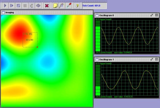
接下來,我們就繼續觀摩一下這個 toolkit 還提供了甚麼:

很明顯地,右邊那兩個綠底、裡面畫有 sine 波的東東,就是示波器(socillograph)的 scope 。比較特別的是這裡的示波器原則上是無限量供應的,只要點選 toolbar 上面代表探針(probe)的 icon 即可。值得一提的還有,這裡的探針量測的不是單純的點的訊號,而是一個指定的範圍。我們可以在左圖的 Imaging 畫布上看到一個虛線框住的範圍,它對應到右上那個 scope ,以這個例子來說,scope 顯示的是整個框框內所有點的平均訊號,實際上我們可以在上面顯示其他更有用的統計。
最後,我這裡也附上 SineSun 的 jar 檔,有興趣的話,諸位看官也可以自行玩玩看 :)